D. REMOVING STELLAR ASTROPHYSICS AND QUARTER STITCHING

Step 1: Stitch quarters of SAP data together

In walk-through's A, B and C, methods for minimizing systematic data artifacts while conserving signal of astrophysical origin were demonstrated. The purpose of walk-through D is to flatten both systamtic artifacts and astrophysical signal in order to fold candidate planet transits successfully upon their orbital period and characterize them with a physical model. The example data comes from the quarter 10 and 11 observations of KIC 12557548. Before execution, the user must create an ASCII file kepstitch.txt which a list of the quarter 10-11 long cadence light curves kplr012557548-2011177032512_llc.fits and kplr012557548-2011271113734_llc.fits, one file per line. The PyKE tool kepstitch appends the quarter 11 time-series light curve to the quarter 10 time-series within the new file kepstitch.fits.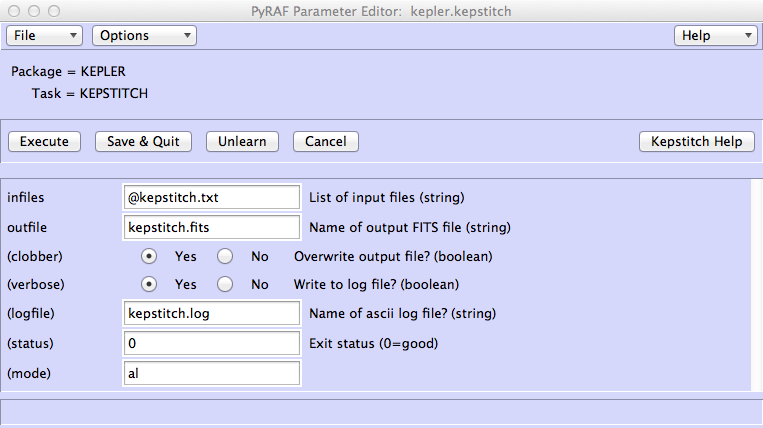

Step 2: Plot stitched PDCSAP data

The quarter-stitched PDCSAP light curve of KIC 12557548 is shown in Figure D1, as rendered by kepdraw.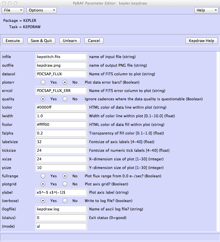

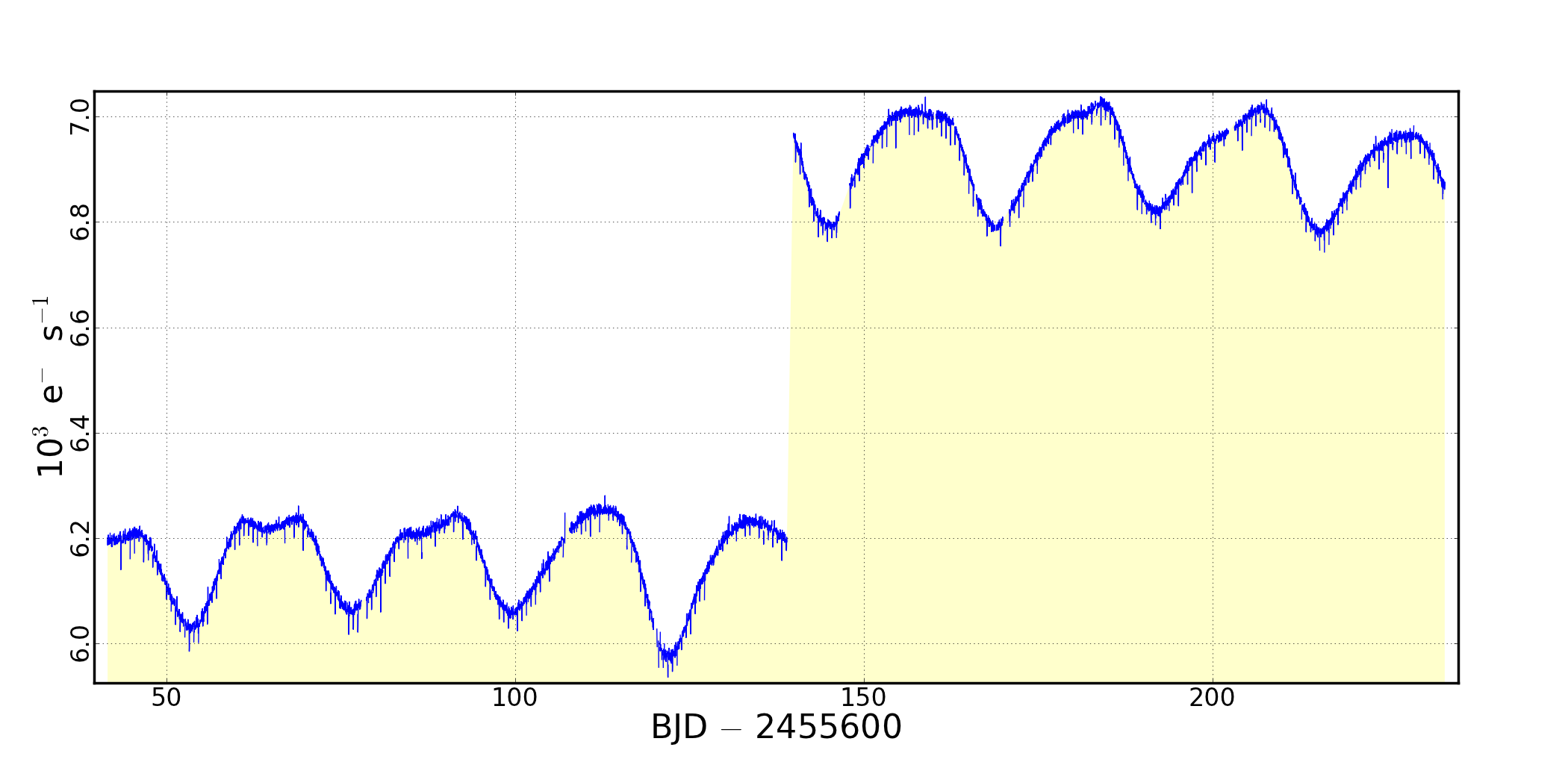
Figure D1: The quarter 10 and 11 long cadence PDCSAP light curves of KIC 12557548. Transit like events recur within this light curve on a 15.6-hr period. Systematic artifacts across individual quarters have been mitigated for to some degree within PDC data. Common to many Kepler time series, the discontinuity is a consequence of different shaped optimal apertures on either side of the quarter gap. Both the stellar astrophysics (rotation on ~20-d timescale) and quarter-gap discontinuity make transit characterization non-trivial.

The delivered command is asking that the PDCSAP_FLUX column in the FITS file kepstitch.fits be plotted to a new file called kepdraw.png. Plotting of the 1-σ error bars from the PDCSAP_FLUX_ERR column is suppressed, and timestamps with non-zero quality flags will be ignored. Additional parameters control the look and feel of the plot – e.g. colors, line widths, fonts, etc. Systematic structure in the form of DVA and thermal trends following monthly data downloads has been mitigated for in the PDC data. This corrected and archived form of the data, or CBV custom-corrected data from the kepcotrend task, are the logical starting point for transit analysis.

Step 3: Flatten quarter 10 PDCSAP data

With systematic artifacts already mostly-removed, the light curves need to be flattened but in a way that does not radically contaminate the transit profile with new systematic structure. The PyKE tool kepflatten fits piecemeal low-order polynomials on small timeslices aross the time-series. Fitting makes user of iterative σ-clipping that removes statistical outliers from a best-fit before refitting until no more time-stamps are rejected. In this way, transits profiles are conserved during the fit process and subsequent normalization by the final best-fit. The flattened are written to the output file in two new columns, DETSAP_FLUX and DETSAP_ERR_FLUX.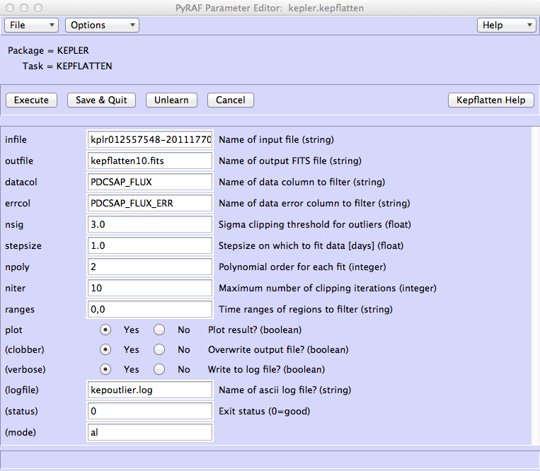

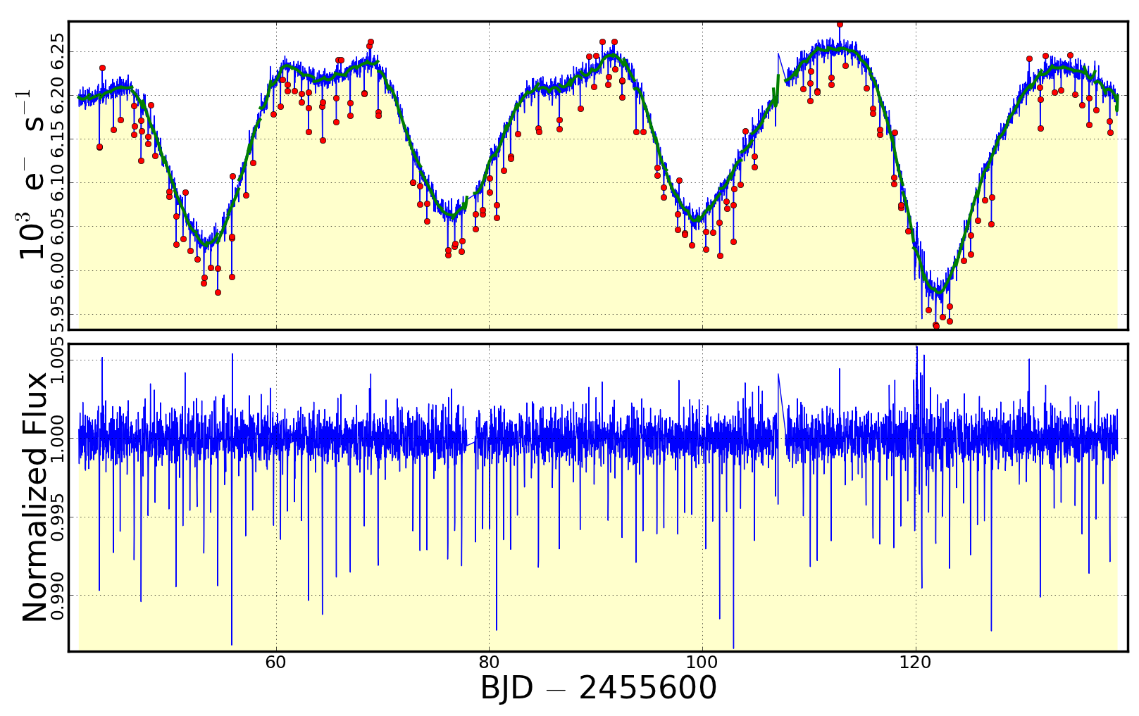
Figure D2: Piecemeal polynomial fit and subtraction of the quarter 10 long cadence PDCSAP data of KIC 12557548. Top: The blue curve is the PDCSAP data. The green curve is the best-fit, piecemeal polynomial. The red dots are the timestamps excluded by the fit through σ-clipping. Bottom: the residual after divinding quarter 10 PDCSAP data by the best fit.

Step 4: Flatten quarter 11 PDCSAP data

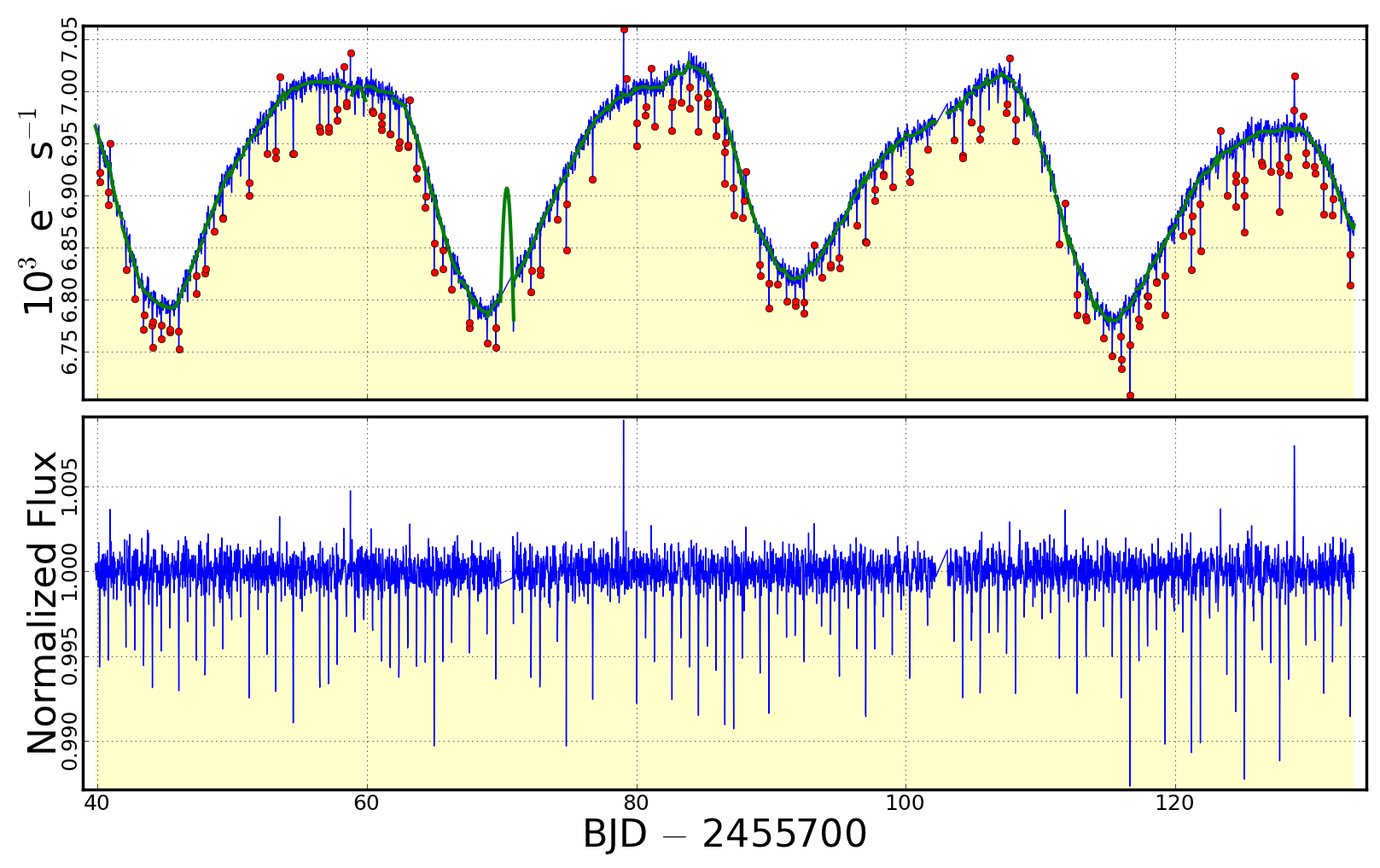
Figure D3: As for Figure D2. Piecemeal polynomial fit and subtraction of the quarter 11 long cadence PDCSAP data of KIC 12557548 using the kepflatten tool.

Step 5: Stitch quarter 10 and 11 flattened data together

Before execution, the user must create the ASCII file kepflatten.txt - a list of the flattened quarter 10-11 long cadence light curves kepflatten10.fits and kepflatten11.fits, one filename per line.

Step 6: Fold flattened and stitched data over the transit period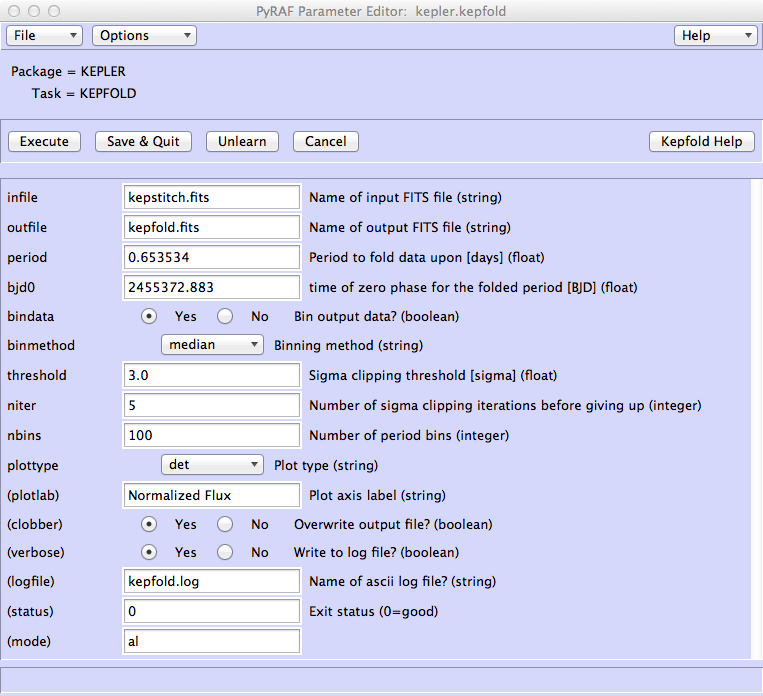

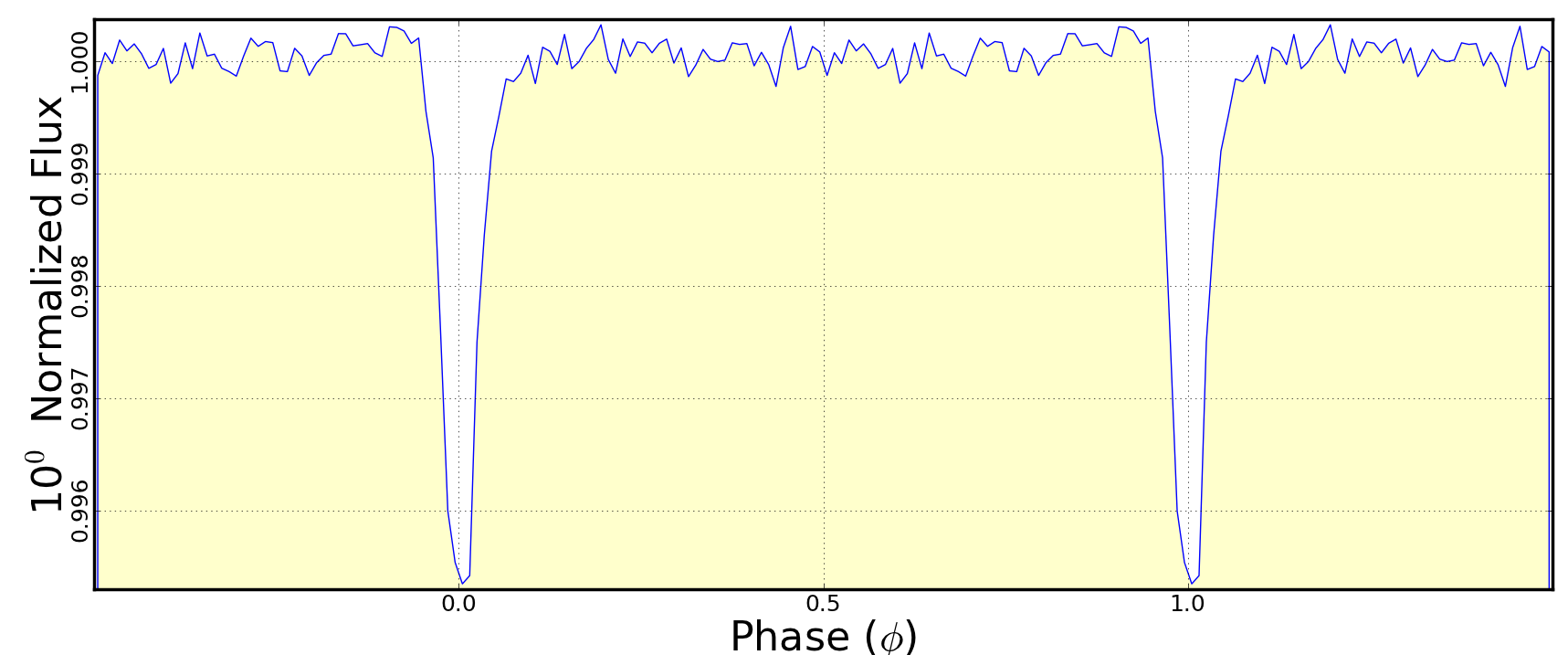
Figure D4: The flattened and stitched Q10-11 PDCSAP light curve of KIC 12557548, folded on a period of 0.653534 days and where zero orbital phase is defined to be BJD 2455372.883. The data was median-averaged into 100 bins across the orbital cycle. Kepler data validation reports indicate that this planet candidate should have a radius of 2.7 R_e, assuming a host star radius of 0.661 R_sun determined from KIC stellar parameters.