C. SUBJECTIVE LIGHT CURVE COTRENDING USING BASIS VECTORS

Step 1: Plot archived SAP data

Kepler's optimal apertures are calculated individually for each target within the pipeline. The calculation assumes that the science of interest occurs on the same timescales as planet transits, mostly < 12-hrs. Walkthrough's A and B provide examples where re-extracting light curves from different sets of pixels improves the quality of data over a broader range of timescales. In many of these cases, systematic artifact removal is then required using the Cotrending Basis Vectors (CBVs). In quiet stars, cotrending Kepler data is often routine. However the more "astrophysics" that occurs within a SAP light curve the greater the danger of astrophysics being fit by a basis vector and removed from the data during the cotrending process. Manual cotrending is a subjective process and this walk-through provides a typical pitfall example and how to navigate it.

In this example we will reduce the systematic trends present in the quarter 3 SAP time-series of an eccentric ('heartbeat') binary star, KIC 3749404. This target provides a test case because the astrophysical model of tidally-driven pulsation and distortion predicts highly-repetitive photometric structure each 20-d binary orbit. As we proceed through the steps, note that each improvement requires a subjective decision based upon both foreknowledge of events recorded in the Kepler data quality flags and physical insight of the target in question. The archived SAP photometry of this target is plotted against barycenter-corrected time in Figure C1. This plot was made using the PyKE tool kepdraw: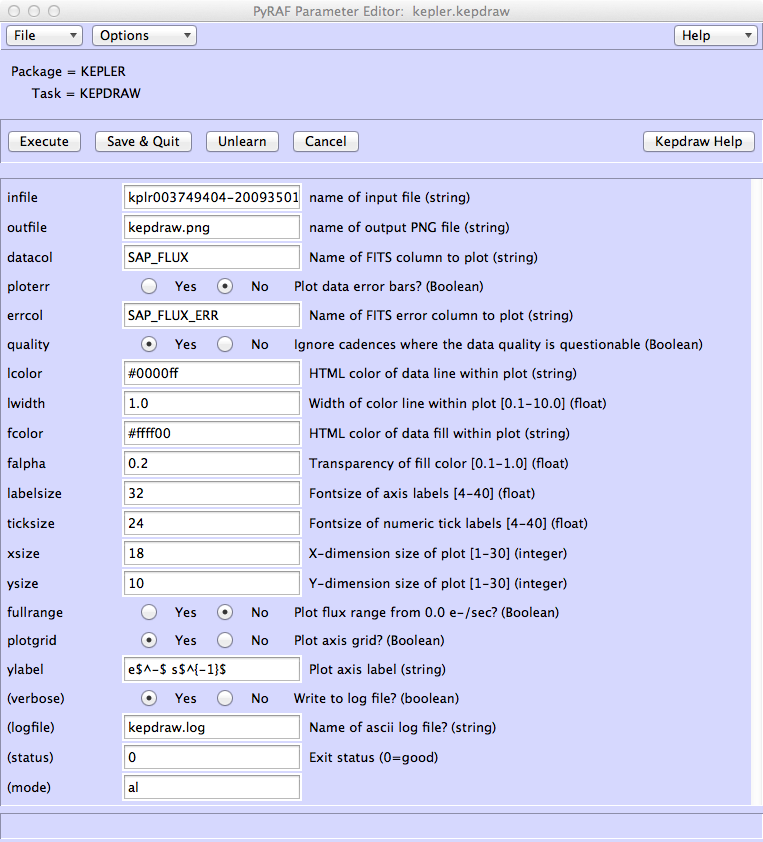

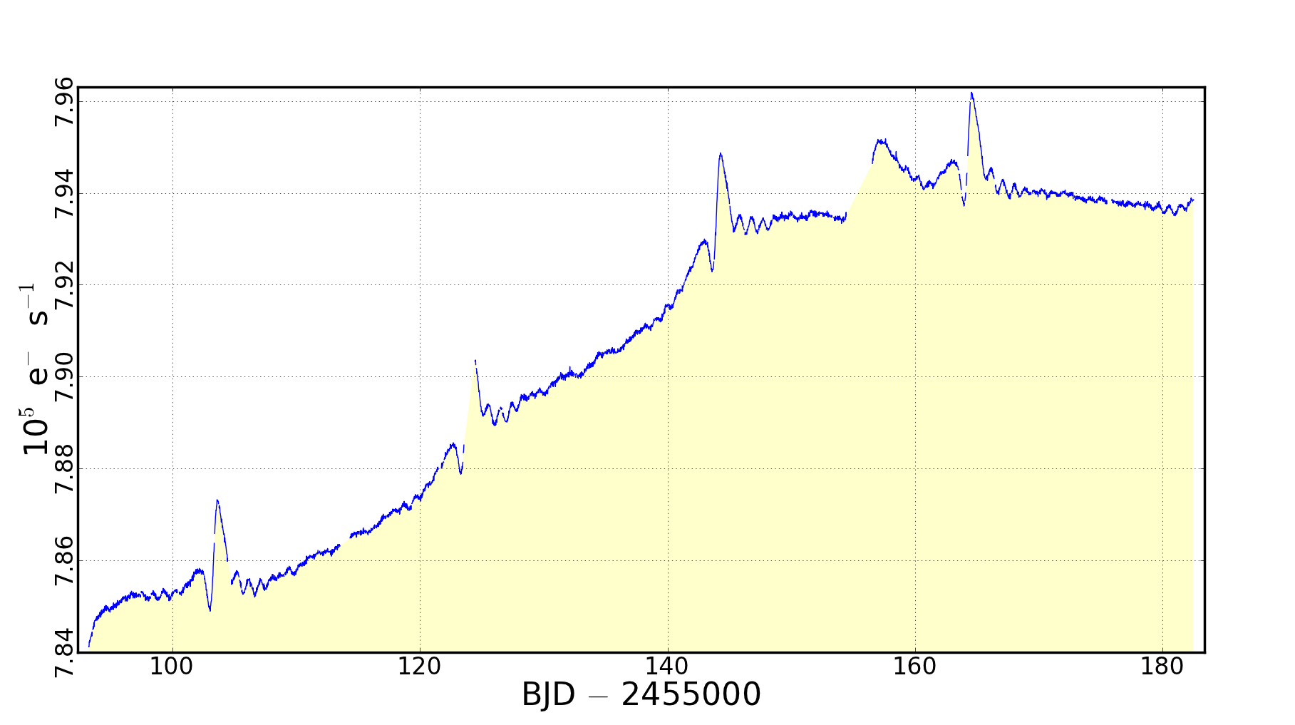
Figure C1: The quarter 3 long cadence SAP light curve of KIC 3749404. The long-term trend of increasing flux, 1% in amplitude, is most-likely caused by differential velocity aberration. A 5-d interval of thermal settling after an Earth point at BJD 2,455,156 stands out as a likely systematic feature over the astrophysical signal.

The delivered command is asking that the SAP_FLUX column in the archived FITS file kplr003749404-2009350155506_llc.fits be plotted to a new file called kepdraw.png. Plotting of the 1-σ error bars from the SAP_FLUX_ERR column is suppressed, and timestamps with non-zero quality flags will be ignored. Additional parameters control the look and feel of the plot – e.g. colors, line widths, fonts, etc. Systematic structure is apparent in the form of DVA and thermal trends following monthly data downloads.

Step 2: Plot archived PDCSAP data

In figure C2, we render the same data after systematic artifact mitigation by the Kepler pipeline's PDC module. The cotrending basis vectors have been fit and subtracted by the PDC module to largely remove systematic structure within the light curve.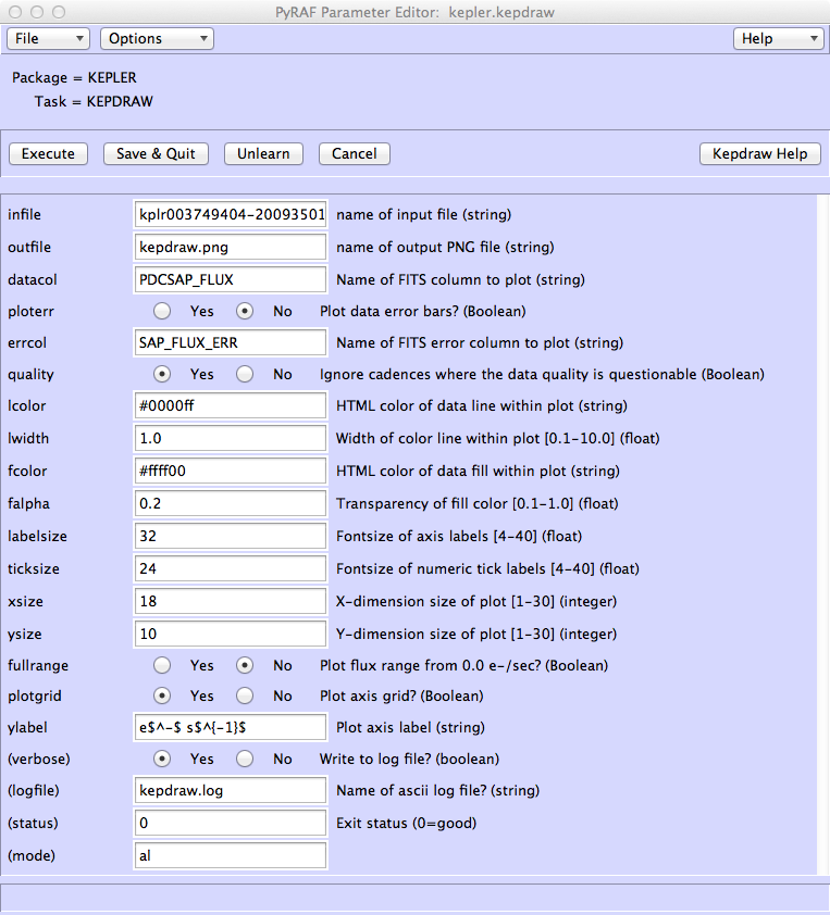

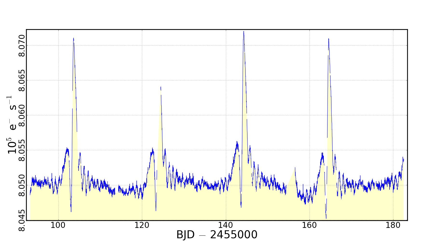
Figure C2: The archived quarter 3 PDCSAP light curve of KIC 3749404.

Step 3: Fit and subtract 2 basis vectors from SAP light curve

To fit the first two quarter 3 CBVs to the quarter 3 data, use the kepcotrend task: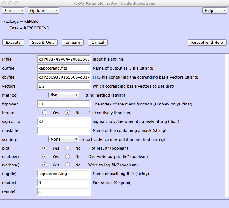

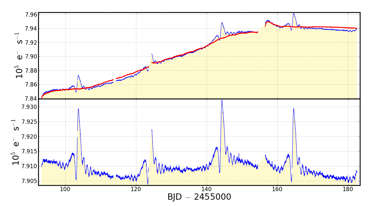
Figure C3: A two-CBV fit to the archived quarter 3 SAP light curve of KIC 3749404. The upper panel of the plot shows the original SAP light curve in blue and the best linear least-squares fit of the two basis vectors in red. The lower plot contains the result of subtracting the best-fit basis vectors from the original light curve. While systematic effects have been reduced, some remain - e.g. between the first and second maxima around BJD 2,455,115.

The llsq method requires kepcotrend to perform a linear least-squares fit and subtraction of the basis vectors from the SAP data. No sigma clipping iterations are performed during the fit. The quarter 3 CBV file, kplr2009350155506-q03-d04 lcbv.fits, can be downloaded from the Kepler archive at MAST. The full content of the input light curve file is copied to the output file and a new column called CBVSAP_FLUX is appended to the FITS table containing the best-fit, CBV-subtracted light curve. The result is shown in Figure C3 and yields an improvement over the photometric quality of the SAP light curve. The long-term trend has been greatly reduced, but there are still higher-frequency features that are most likely systematic, and the fit can be improved further.

Step 4: Fit and subtract 5 basis vectors from SAP light curve

Performing another fit using five basis vectors with the following command yields the result shown in Figure C4. Provided the user specifies clobber=yes, any pre-existing file called kepcotrend.fits will be over-written by the output from this step. The task will stop with a warning if a pre-existing file called kepcotrend.fits exists and clobber=no. This new result is a qualitative improvement compared to the two-CBV fit, but the solution is still does not approach the orbit-repeatibility found in the archived PDCSAP light curve in Figure C2.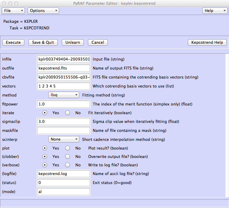

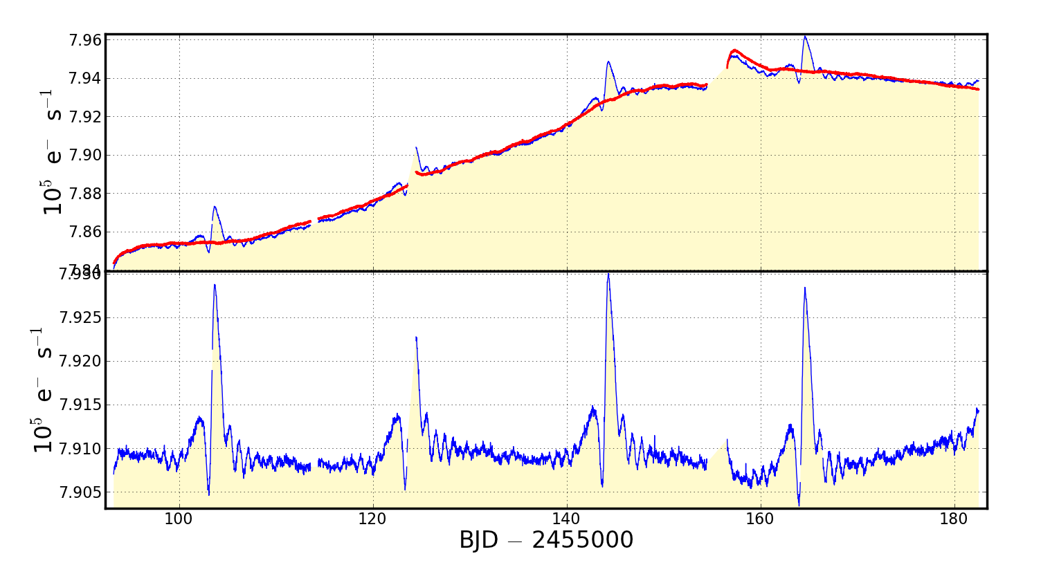
Figure C4: As for Figure C3 but this time five CBVs are fit to the quarter 3 SAP light curve of KIC 3749404. The systematics now appear to be much reduced but there are still some effects in the second half of the quarter that can be mitigated further (e.g. the fit to the thermal settling event around BJD 2,455,156). The quality of systematic mitigation does not yet approach the archived PDCSAP light curve in Figure C2.

Step 5: Fit and subtract 8 basis vectors from SAP light curve

A further fit the SAP data, this time using eight basis vectors is rendered in Figure C5, but the result appears to be less optimal than the 5 basis vector fit. Anomalous structure has been added to the resulting time series by high-order CBVs. Least-square fitted CBVs never approach the archived PDCSAP data regardless of the number of CBVs in the fit ensemble. Eight basis vectors are over-fitting the periodic bright events and adding new systematic noise to the intervals between them. The pipeline PDC module combats many such situations in the Kepler archive by fitting CBV coefficients simultaneously to the target and a sample of target near-neighbors on the detector plane. The quietest targets in the locality provide the greatest weight in the fit minimization. The PyKE approach is different - rather than analyzing target samples, PyKE provides the flexibility to tune data reduction to target specific data quality and science optimization. In the PyKE paradigm, users have the ability to try different fit minimization methods, reject photometric outliers and ignore individual timestamps during fit minimization.

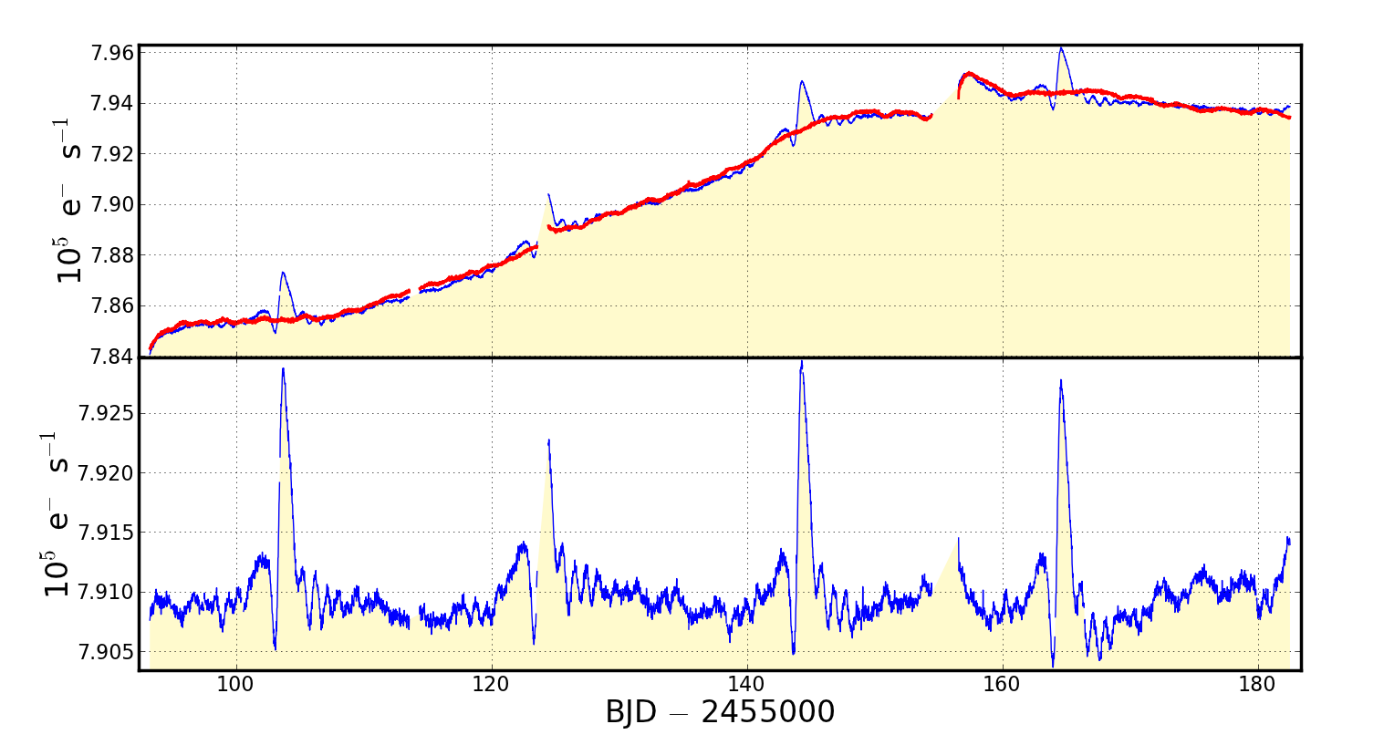
Figure C5: As for Figures C3 and C4. This fit to the quarter 3 SAP light curve of KIC 3749404 contains eight basis vectors and appears to be performing less well than a five basis vector fit and the archived PDCSAP time-series.

Step 6: Select time intervals to be ignored during cotrending

The quality of the CBV fit will improve if we mask time intervals of rapid astrophysical variability. Masked intervals are defined using the task keprange. This will plot the SAP FLUX column data within the light curve file over time. Ranges in time can be defined by selecting start and stop times with the mouse and ’X’ keyboard key. We masked four ranges in this example and these ranges will be saved to a text file after clicking the ‘SAVE’ button on the interactive GUI.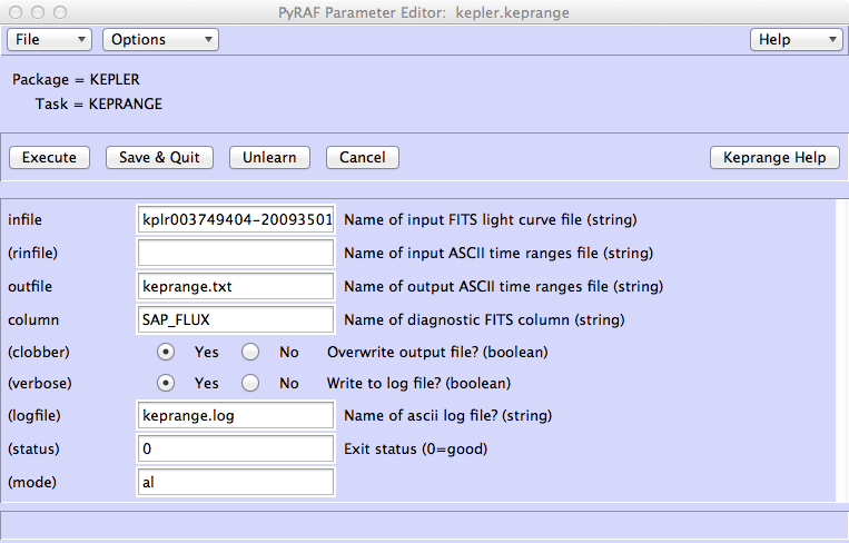

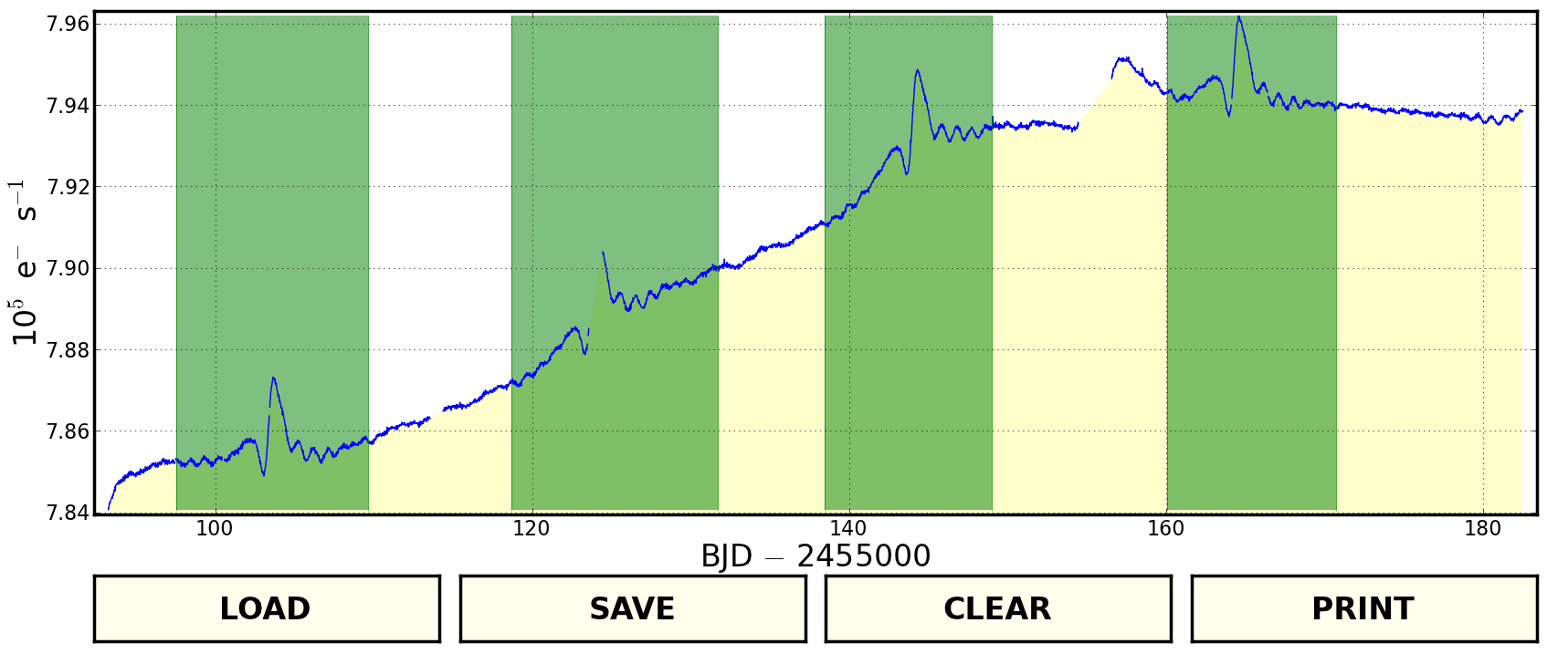
Figure C6: This figure renders the interactive environment of the keprange tool, developed to define and store discrete intervals of time-series data. The timestamps inside the green highlighted regions will be excluded from the fit during the final run of kepcotrend in Step 7.

Step 7: Fit and subtract 8 basis vectors from SAP light curve with filtering

We performed the eight basis vector fit one last time, excluding from the fit the regions defined in Figure C6, again using the kepcotrend task. In terms of repeatibility, an individually-filtered call to kepcotrend has provided an improvement in quality over the pipeline's PDC module (Figure C2). The most conspicous remaining artifacts coincide with the thermal settling events after each of the three Earth-points during the quarter. Continued development on the pipeline and construction of the archived CBVs is addressing these features.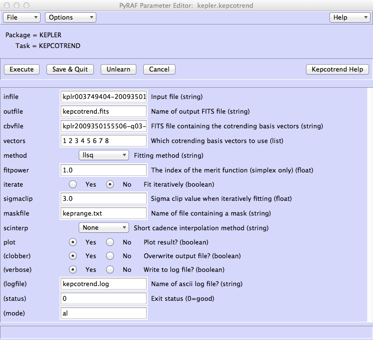

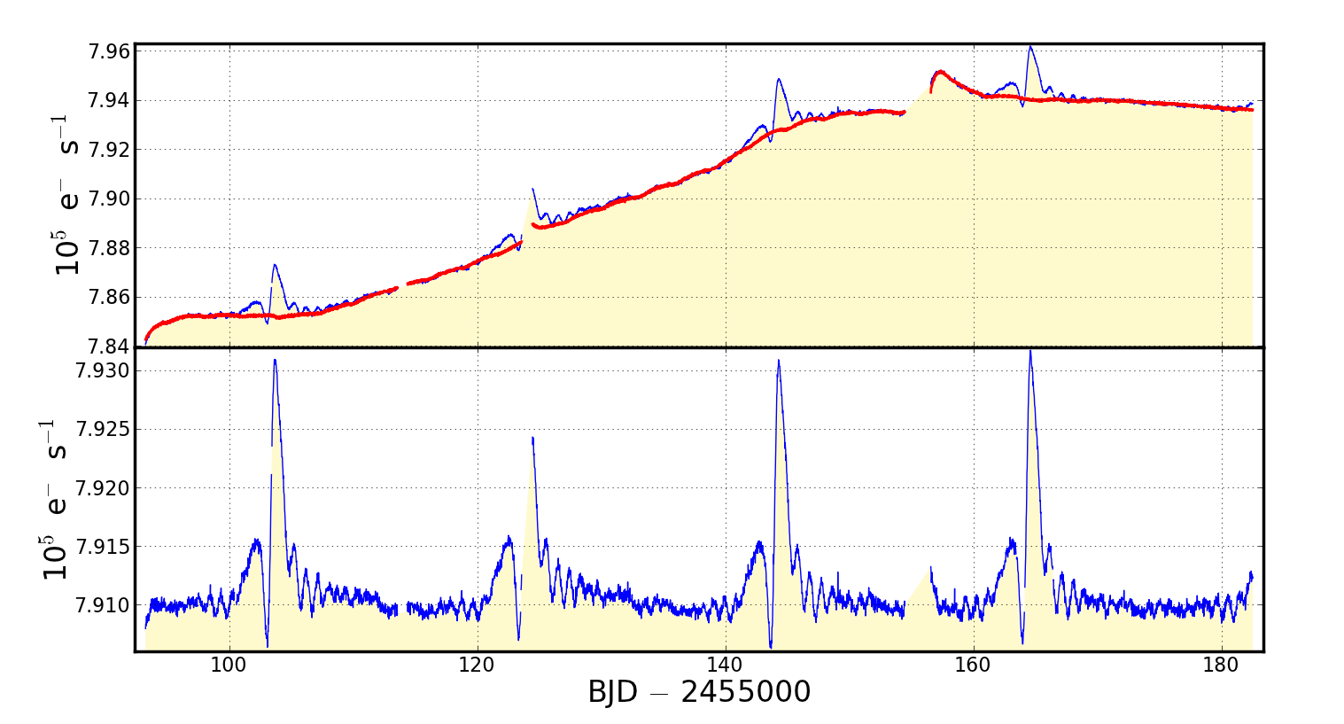
Figure C7: The final iteration of the CBV fit to the quarter 3 SAP light curve of KIC 3749404 using the PyKE tool kepcotrend, fitting eight basis vectors. The regions of the light curve highlighted green in Figure C6 were excluded from the fit.