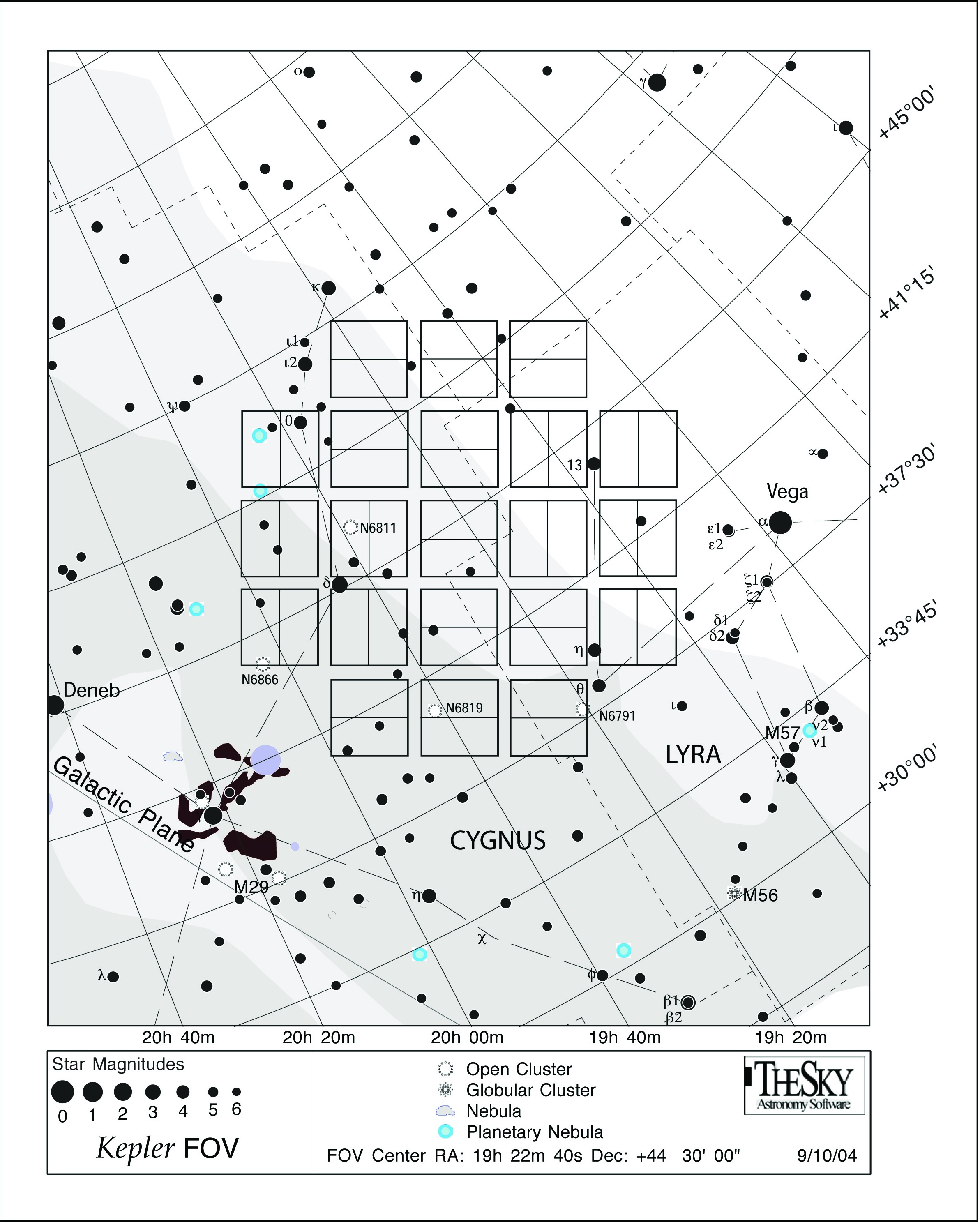
LIGHT CURVE INSPECTION WITH TOPCAT

Kepler times-series light curves are provided to the user in the form of a binary FITS table, one file per target. Each row in the table contains timestamps, photometric measurements, astrometric measurements and data quality flags. A format description and content definition of the Kepler light curve file is provided in section 2.3.1 of the Kepler Archive Manual. We provide a specific example of light curve product inspection using the Java tool TOPCAT. After starting up the TOPCAT application, the main control GUI will open (figure 1). The left-most icon on the options bar at top allows the user to open and inspect light curve files. Other icons provide data table display, data plotting, filtering and statistics, and output of a variety of different data formats.

i) LOAD DATA

• Clicking on the "Load New Table" icon (top-left) will open a new GUI. In the "Format" dialog box scroll down and click on "FITS".
• Click on the "Filestore Browser" button to navigate through your directories; choose the desired file by clicking on it.
• The file name will appear in the left-hand window of the main GUI. The number of rows and columns in the table will appear in the right-hand area.

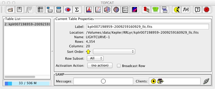
Figure 1: TOPCATs main control GUI. Data I/O and display options are performed by mouse-clicking the icons across the top. When the mouse hovers over the icon, a brief description of the button is provided. The left-hand pane lists opened files; the right-hand pane displays information about the currently selected file.

ii) DISPLAY DATA TABLE

• Clicking the fourth icon from the left in the primary GUI opens the data table within the FITS file for inspection, like the one below.

Figure 2: Typical data table from an archived light curve product, as displayed by the TOPCAT software. Column headings are provided at the top of the table.

iii) PLOT DATA TABLE

• Click on the icon labeled "Scatter Plot" at the top of the control window. A plotting GUI opens in which data in the TIME column (col. 1) is plotted versus data in the TIMECORR column (col. 2), the default option.
• In the plot window, the user can select alternative data columns to plot. For the Y-axis data choose, for example the data column SAP_FLUX. The plot will update with simple aperture photometry against time.
• Options for customizing the plot are available using the various icons located above the plot. For example:
  • Axis titles and XY scale ranges are set using the 3rd icon along the top of the GUI.
  • Rescale the plot using the arrow icons.
  • At the bottom right of the plot, under "Row Subsets", click on the rightmost button, to access the Plot Style Editor.
• Save the plot to PDF using icon 4.

Figure 3: TOPCAT plot of calibrated simple aperture photometry vs barycentric Julian Date. This sequence of data is RR Lyr observed through Q2.

---

iv) SAVE DATA TABLE TO ASCII

• Convert data to e.g. ASCII files, using the "Save Table" option - the second icon from the left at the top of the control window.