Software: PyKE
Version: 3.0.1
Contributor:

NAME
kepcotrend -- Remove systematic trends Kepler light curves using cotrending basis vectors

USAGE
kepcotrend infile outfile cbvfile vectors method fitpower iterate sigmaclip maskfile plot clobber verbose logfile status

PARAMETERS
infile = string
The name of a MAST standard format FITS file containing a Kepler long or short cadence light curve within the first data extension.

outfile = string
The name of the output FITS file. outfile will be an amended version of infile with two extra columns called CBVSAP_MODL and CBVSAP_FLUX. These columns contain the linear sum of cotrending basis vectors removed from the simple aperture photometry flux and newly calculated flux with the cotrending basis vector sum removed, respectively.

cbvfile = string
The name of the FITS file containing the cotrending basis vectors data which will be used to cotrend away systematic errors in the data. These files are stored, one for each Kepler quarter, at the MAST Archive and can be downloaded directly. The file name will be in the format kplr<yyyydddhhmmss>-q<nn>_lcbv.fits <yyyydddhhmmss> corresponds to the last cadence of the quarter, named the same as the light curve and target pixel files. <nn> is a 2 digit integer for the quarter. lcbv refers to Long cadence Cotrending Basis Vectors.

vectors = string
The sequence of cotrending basis vectors are fit to the data. The input format for this is a list of integers separated by either a space, comma, colon, semi-colon or pipe character. Each number specifies a basis vector to include in a fit to the input light curve. For example to use the first four basis vectors the input would be '1 2 3 4', and to use components one through five excluding two and three: '1 4 5'. It is strongly recommended that at least two basis vectors are used.

method = string
The Method used to fit the linear sum of cotrending basis vectors to the light curve. The options are: llsq and simplex.

1. llsq is a linear least squares fit and is the most CPU-efficient method: a least squares fit is the equivalent of multiplying the inverse product of the transpose matrix of the basis vectors and the matrix of the basis vectors with the product of the transpose matrix of the basis vectors and the light curve time series. In mathematical form this is [U^T * U]^-1 * U^T * y, where y is the light curve flux time series and U is the matrix of basis vectors.
2. simplex uses the Nelder-Mead downhill simplex method.

fitpower = string
When using the simplex fitting method, the function that is minimized (the merit function) takes the form abs(observed - fit)^P where the index P is fitpower. For a least squares fit P=2 and for a least absolute difference P=1.
Acceptable results usually come from using the llsq method but the simplex method will produce differing best solutions if P != 2. This can be desirable when the best least squares solution is too sensitive to astrophysical variability that the user wants to retain. Lowering the value of P often provides better results for highly variable targets. It is the users responsibility to decide which method provides a best solution.

iterate = boolean
Whether to fit the basis vectors data iteratively, clipping data points further than sigmaclip from the best-fit curve and redoing the fit without the clipped data points. All three fitting methods can be performed iteratively. The code iterates a maximum of 50 times. This parameter is ignored if method=llsq.

sigmaclip = string
If iterate=yes, when a data point is more than ±sigmaclip from the best fitting linear combination of basis vectors then that point is excluded from subsequent fit iterations.

maskfile = string
The best best basis vector fit can interpret photometric features as a combination of basis vectors rather than as intrinsic variability from the target, providing an undesirable cotrending solution. This is common for example when a target undergoes a temporary but large state change, e.g. the outburst of a cataclysmic variable. It is possible to mask regions of the light curve from being included in the fit to the light curve. The mask file is in the format that is created using the keprange tool. When choosing to mask regions from the fit, give the filename here, otherwise leave the field blank, i.e. ''.

scinterp = string
The basis vectors are only calculated for long cadence data. Using short cadence data requires interpolation of the basis vectors. We have implemented several methods of interpolation: linear, nearest, slinear, quadratic and cubic. We recommend nearest interpolation which will fit the each short cadence data-point to the associated long cadence basis vector data-point.

plot = boolean
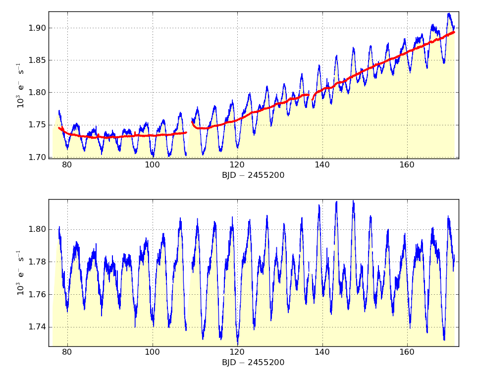
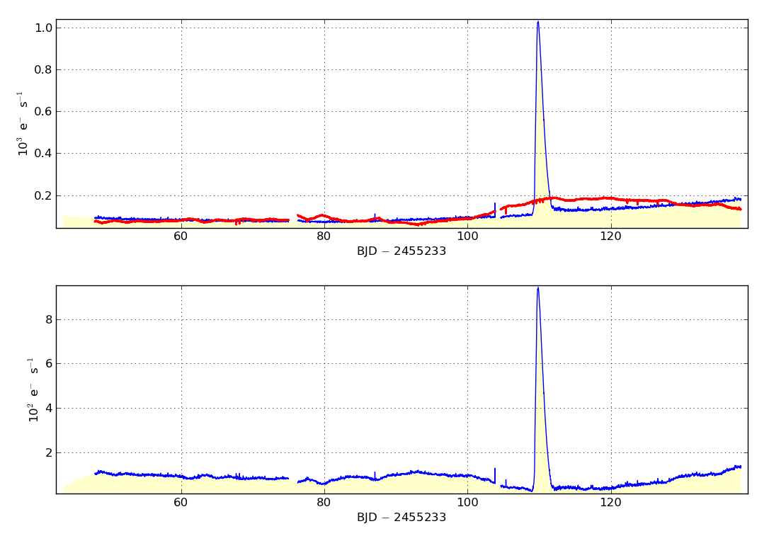
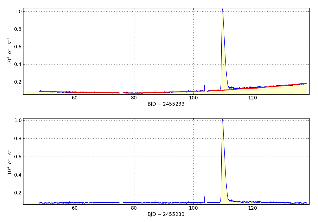
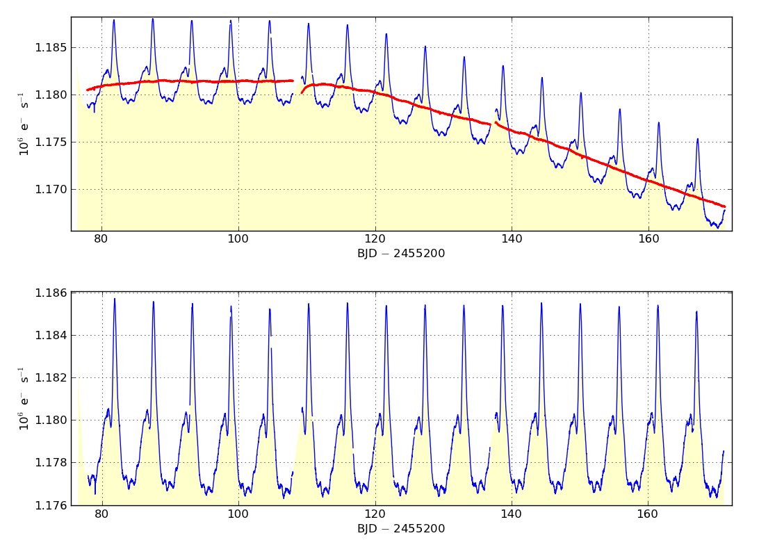
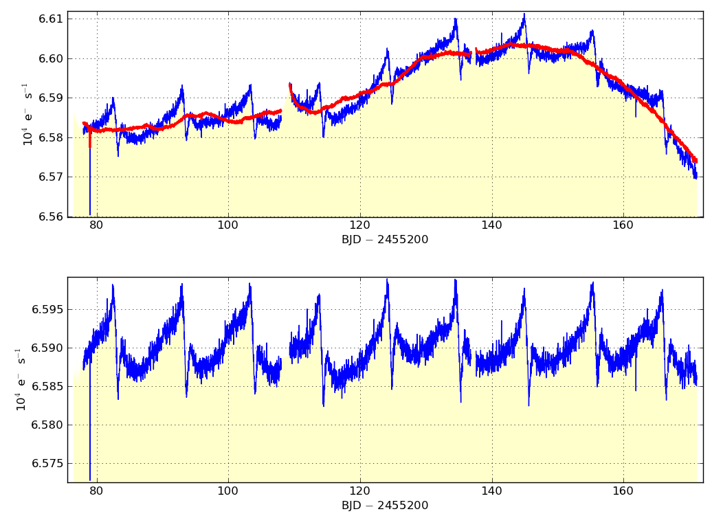
Display results. The plot consists of two panels: the top panel shows the SAP light curve in blue and the best fitting linear combination of cotrending basis vectors in red. The lower panel shows the result of subtracting the sum of basis vectors from the SAP time series.

clobber = boolean (optional)
Overwrite the output file? if clobber = no and an existing file has the same name as outfile then the task will stop with an error.

verbose = boolean (optional)
Print informative messages and warnings to the shell and logfile?

logfile = string (optional)
Name of the logfile containing error and warning messages.

status = integer
Exit status of the script. It will be non-zero if the task halted with an error. This parameter is set by the task and should not be modified by the user.

DESCRIPTION
Simple Aperture Photometry (SAP) data often contain systematic trends associated with the spacecraft, detector and environment rather than the target. See the the Kepler data release notes for descriptions of systematics and the cadences that they affect. Within the Kepler pipeline these contaminants are treated during Pre-search Data Conditioning (PDC) and cleaned data are provided in the light curve files archived at MAST within the column PDCSAP_FLUX. The Kepler pipeline attempts to remove systematics with a combination of data detrending and cotrending against engineering telemetry from the spacecraft such as detector temperatures. These processes are imperfect but tackled in the spirit of correcting as many targets as possible with enough accuracy for the mission to meet exoplanet detection specifications.

The imperfections in the method are most apparent in variable stars, those stars that are of most interest for stellar astrophysics. The PDC correction can occasionally hamper data analysis or, at worst, destroy astrophysical signal from the target. While data filtering (kepoutlier, kepfilter) and data detrending with analytical functions (kepdetrend) often provide some mitigation for data artifacts, these methods require assumptions and often result in lossy data. An alternative viable approach is to identify the photometric variability common to all of the stars neighboring the target and subtract those trends from the target. In principle, the correct choice, weighting and subtraction of these common trends will leave behind a corrected flux time series which better represents statistically the true signal from the target.

While GOs, KASC members and archive users wait for the Kepler project to release quarters of data, they do not have access to all the light curve data neighboring their targets and so cannot take the ensemble approach themselves without help. To mitigate this problem the Kepler Science Office have made available ancillary data which describes the systematic trends present in the ensemble flux data for each CCD channel. These data are known as the Cotrending Basis Vectors (CBVs). More details on the method used to generate these basis vectors will be provided in the Kepler Data Processing Handbook soon, but until that time, a summary of the method is given here. To create the initial basis set, that is the flux time series' that are used to make the cotrending basis vectors:

1. The time series photometry of each star on a specific detector channel is normalized by its own median flux.
2. One (unity) is subtracted from each time series so that the median value of the light curve is zero.
3. The time series is divided by the root-mean square of the photometry.
4. The correlation between each time series on the CCD channel is calculated using the median and root-mean square normalized flux.
5. The median absolute correlation is then calculated for each star.
6. All stars on the channel are sorted into ascending order of correlation.
7. The 50 percent most correlated stars are selected.
8. The median normalized fluxes only (as opposed to the root-mean square normalized fluxes) are now used for the rest of the process
9. Singular Value Decomposition is applied to the matrix of correlated sources to create orthonormal basis vectors from the U matrix, sorted by their singular values.
10. The archived cotrending basis vectors are a reduced-rank representation of the full set of basis vectors and consist of the 16 leading columns.

To correct a SAP light curve, F_sap, for systematic features, kepcotrend employs the cotrending basis vectors CBV_i. The task finds the coefficients A_i which minimize

F_cbv = F_sap - Σ_i (A_i . CBV_i)

The corrected light curve, F_cbv, can be tailored to the needs of the user and their scientific objective. The user decides which combination of basis vectors best removes systematics from their specific Kepler SAP light curve. In principle the user can choose any combination of cotrending basis vectors to fit to the data. However, experience suggests that most choices will be to decide how many sequential basis vectors to include in the fit, starting with first vector. For example a user is much more likely to choose a vector combination 1, 2, 3, 4, 5, 6 etc over e.g. a combination 1, 2, 5, 7, 8, 10, 12. The user should always include at least the first two basis vectors. The number of basis vectors used is directly related to the scientific aims of the user and the light curve being analyzed and experimental iteration towards a target-specific optimal basis set is recommended. Occasionally kepcotrend over-fits the data and removes real astrophysical signal. This is particularly prevalent if too many basis vectors are used. A good rule of thumb is to start with two basis vectors and increase the number until there is no improvement, or signals which are thought to be astrophysical start to become distorted.

The user is given a choice of fitting algorithm to use. For most purposes the llsq method is both the fastest and the most accurate because it gives the exact solution to the least squares problem. However we have found a few situations where the best solution, scientifically, comes from using the simplex fitting algorithm which performs something other than a least squares fit. Performing a least absolute residuals fit (fitpower=1.0), for example, is more robust to outliers.

There are instances when the fit performs sub-optimally due to the presence of certain events in the light curve. For this reason we have included two options which can be used individually or simultaneously to improve the fit - iterative fitting and data masking. Iterative fitting performs the fit and rejects data points that are greater than a specified distance from the optimal fit before re-fitting. The lower threshold for data clipping is provided by the user as the number of σ from the best fit. The clipping threshold is more accurately defined as the number of Median Absolute Deviations (MADs) multiplied by 1.4826. The distribution of MAD will be identical to the distribution of standard deviation if the distribution is Gaussian. We use MAD because in highly non-Gaussian distributions MAD is more robust to outliers than standard deviation.

The code will print out the coefficients fit to each basis vector, the root-mean square of the fit and the chi-squared value of the fit. The rms and the chi-squared value include only the data points included in the fit so if an iterative fit is performed these clipped values are not included in this calculation.

EXAMPLE

• Example #1 - a rapid rotator with evolving spots:
  kepcotrend infile=kplr005110407-2009350155506_llc.fits outfile=new1.fits cbvfile=kplr2009350155506_Q3_lcbv.fits vectors='1 2 3 4 5' method=llsq fitpower=None iterate=n sigmaclip=None maskfile='' scinterp='None' plot=y clobber=y
  
• Example #2a - poor fit with no data masking:
  kepcotrend infile=kplr004937206-2009350155506_llc.fits outfile=new2.fits cbvfile=kplr2009350155506-q03-d04_lcbv.fits vectors='1 2 3 4 5 6 7' method=llsq fitpower=None iterate=n sigmaclip=None maskfile='' scinterp='None' plot=y clobber=y
  
• Cotrending example #2b - good fit with masking of the bright photometric outburst at BJD 2455343:
  kepcotrend infile=kplr004937206-2009350155506_llc.fits outfile=new3.fits cbvfile=kplr2009350155506-q03-d04_lcbv.fits vectors='1 2 3 4 5 6 7' method=llsq fitpower=None iterate=n sigmaclip=None maskfile=keprange.txt scinterp='None' plot=y clobber=y
  
• Example #3: kepdetrend infile=kplr012455116-2009350155506_llc.fits outfile=new4.fits cbvfile=kplr2009350155506-q03-d04_lcbv.fits vectors='1 2' method=llsq fitpower=None iterate=n sigmaclip=None maskfile='' scinterp='None' plot=y clobber=y
  

Example #4 with iterative sigma clipping: kepdetrend infile=kplr011125706-2009350155506_llc.fits outfile=new5.fits cbvfile=kplr2009350155506-q03-d04_lcbv.fits vectors='1 2 3 4 5 6 7 8' method=llsq fitpower=None iterate=y sigmaclip=2.5 maskfile='' scinterp='None' plot=y clobber=y

TIME REQUIREMENTS
Full completion upon one quarter of Kepler long cadence target using a 3.06 GHz Intel Core 2 Duo Mac running OS 10.6.4 takes a few seconds. Using short cadence data an interpolating using a quadratic or cubic function can take several minutes.

SOFTWARE REQUIREMENTS
This tool requires having a numpy version of at least 1.4 to run because kepcotrend uses the function in1d. Installing the STSCI Python packages is sufficient to run this tool.

BUGS AND LIMITATIONS
kepcotrend now supports Kepler short cadence data. There are not sufficient short cadence targets on each detector channel to build short cadence-specific basis vectors so the vector fitting within kepcotrend interpolates the long cadence basis vectors. This processing will not mitigate for photoemtric systematics within short cadence data that occur on timescales shorter than 30 min, but will mitigate systematic on timescales longer than 30 min.
Basis vector fitting of quarter 2 data can often yield unsatisfactory results due to the two tweaks to spacecraft attitude performed during this quarter. We are developing a solution which allows the user to split the basis vectors into three segments, with splits occurring at the times of the attitude tweaks. These three section of basis vectors will then be fit independently. We hope to include this development in the next version of the software.
The Kepler PyRAF package is privately-developed software made available to the community through the contributed software page of the GO program at http://keplergo.arc.nasa.gov/ContributedSoftware.shtml. It is not an official software product of the Kepler mission. Bugs and errors are not the responsibility of NASA or the Kepler Team. Please send bug reports and suggestions to keplergo@mail.arc.nasa.gov.

HISTORY

Date	Version	Description
2011-07-28	1.0.0	Initial software release (TB)
2011-09-06	1.0.1	Updated the simplex fitting method to improve stability when using large numbers of basis vectors. Code now catches user having old version of numpy without in1d. Added line to code to fix plot not drawing (TB).
2011-10-05	2.0	Kepcotrend can now remove systematic artifacts on timescales > 30 min from short cadence data by interpolating the long cadence basis vectors over the short cadence time stamps. (TB).
2012-03-14	2.01	Fixed a bug in the parameter file whereby it was not excepting 'None' for the scinterp parameter. (TB).
2012-03-27	3.0.0	Code can now be run from the command line (TB)
2012-06-07	3.0.1	more reliable plot rendering on linux operating systems (MS)

SEE ALSO
keprange