Update (July 2007): The KI team has investigated and
quantified a flux bias in the visibility amplitude (see the
flux bias memo for more details). This bias can be
corrected using the -fluxBias command line option in wbCalib and
nbCalib
and we recommend that all KI data be calibrated with this option.
What is data calibration?
The visibility that KI measures on an astronomical object (Vm) is the product of the true object (Vt) visibility and a factor, called the system visibility (Vs), which represents the loss of coherence due to instrumental and atmospheric factors: Vm = Vt * Vs. In order to obtain the true object visibility, the system visibility must be estimated. The system visibility can be estimated using observations of stars of known size, and thus of known true visibility; or more typically using observations of unresolved stars, which have a true visibility of 1.0 and directly provide an estimate of the system visibility (Vm = Vs). Once the system visibility has been estimated, the calibrated or true object visibility is simply obtained as: Vt = Vm/Vs. (Note: the Keck Interferometer data reduction method uses visibility amplitude squared, rather than visibility amplitude, as the basic observable; a distinction with no consequences to the present discussion).
In general the system visibility is an instantaneous quantity, and may depend on other factors such as the object location in the sky (e.g. as the zenith angle increases, the atmospheric effects may become more severe) and the instrument configuration (e.g. integration time). Insuring that target and calibrators can be observed under the same instrument configuration (e.g. have similar magnitudes for the different sub-systems) and are close in the sky, is part of the planning process. Insuring that a target observation is bracketed by calibrator observations with a few minutes cycle time, so that a valid estimate of the system visibility can be formed, is the responsibility of the WMKO/NExScI staff executing the schedule.
How to calibrate your data
Although data calibration is not
performed at the NExScI, we make
available two software packages, wbCalib
(for calibration of
wide-band data) and nbCalib
(for calibration of
narrow-band data), which which greatly automate and simplify this
process. The Calib packages take as input a L1 data file and a calibration
script detailing which objects are targets and which
are calibrators, and their estimated sizes, and produces one file of
Troubleshooting your calibrated data
Once you have calibrated your visibilities, there are some simple checks you can do to insure that they are sensible:- Plot the system visibility, it should be a smoothly varying function, with an average value between 0.6 and 0.8. The system visibility can change with time, for example it may decrease as the zenith angle increases, but abrupt changes are usually indicative of an instrument problem. In that case, inspect your data and observing logs.
- Note that if the calibrators are not unresolved, it is crucial to provide good estimates of their sizes in order to obtain a good estimate of the system visibility. A common way to verify this is to treat a calibrator as a target, and verify that you get the expected value of the calibrated visibilities (for example 1.0 for an unresolved calibrator). If not, then the calibrator sizes may need to be corrected.
Extracting astrophysical information from your calibrated data
Example
Suppose you have just retrieved your L1 data, containing some observations of one of your targets. The wide-band raw visibilities might look as in the plot below: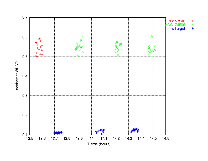
Clearly the above data shows that the source myTarget is clearly resolved, as its raw visibilities are much lower than those of the two calibrators used (HD157546 and HD174596).
The calibration script
# Example calibration script for myTarget

myTarget

17 56 21.288 -21 57 21.880 -0.009 -0.040 0.01

---

2

HDC157546 17 24 37.040 -18 26 44.743 0.016 -0.008 0.02 0.17 0.1

HDC174596 18 52 08.375 -21 55 17.498 0.048 -0.048 0.01 0.21 0.1
Note that the getCal package contains a function that facilitates the generation of properly formatted calibration scripts.
Please pay particular attention to your choice of calibrator angular sizes and errors, as those will directly impact the resulting calibrated visibilities. While for observation planning it is acceptable to provide only approximate calibrator angular sizes, it is crucial to provide accurate estimates with realistic errors in the calibration step. Recall that in addition to providing stellar size estimates based on standard lookup tables for normal stars, the getCal package also contains routines to provide better estimates by fitting spectro-photometric data, see the getCal documentation for details.
Running wbCalib
If we save the above calibration script in a file called "example.calScript", and the L1 SUM data is in a file called "example.sum", then the command to run the calibration program would be:wbCalib -WL -ratioCorrection example.calScript
example.sum >
example.wbcalib
A variery of command line options are available for both wbCalib and nbCalib. The NExScI science team has evaluated these options for KI data, and documented the recommended Calib settings. Note that the recommended settings for KI and PTI are not the same.
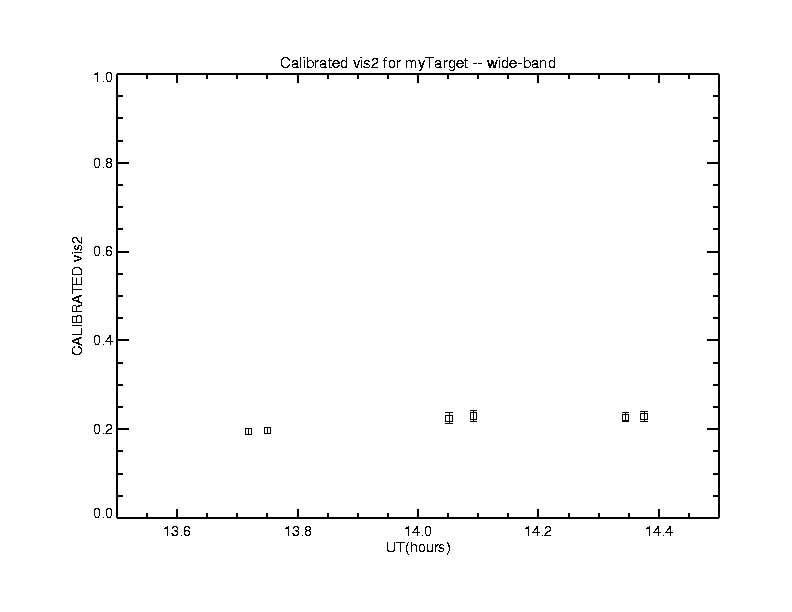
In the example above, we have told wbCalib that we want to use data from the white-light pixel, and to apply a correction for un-balanced fluxes between the interferometer arms. The calibrated data is now in the ASCII file called "example.wbcalib". Please see the wbCalib documentation for a detailed description of the output file fields. Using this file, a plot of the calibrated visibilities and errors versus UT time (columns 8, 9 and 5 respectively) is shown below:
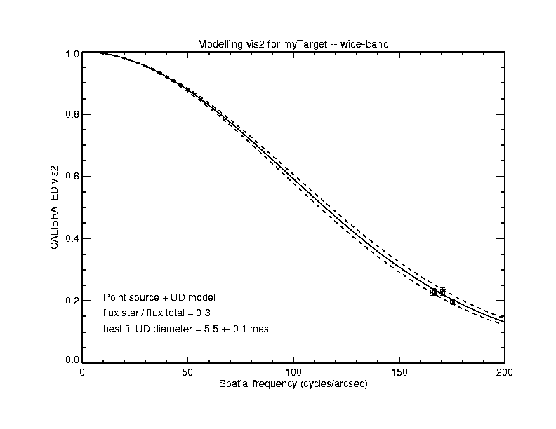
Modelling the calibrated data